TOI 270 exploration
TOI-270 is a very interesting planetary system composed (as far as we know) of one super-Earth, and two mini-Neptunes orbiting an M3V-type star. The discovery paper can be found here:
However, let us imagine that this paper has not been published yet, and you want to recover the signals issued by TESS and/or search for additional planets in the system. The SHERLOCK’s PIPEline is the perfect tool for that.
What we know about it?
In a normal case, if you want to recover the signals described in a TESS release, you may consult the EXOFOP site where you can check the details of the alert.
In this particular case, you would see three alerts for the candidates: .01, .02, and .03, with orbital periods of 5.66, 11.38 and 3.36 days, respectively. The SNRs of the detections were: 41.59, 11.38, and 14.36.
The user-properties.yaml
We only need to prepare our user parameter file, where we specify the TIC ID and a few other parameters:
######################################################################################################################
### GLOBAL OBJECTS RUN SETUP - All sectors analysed at once
######################################################################################################################
###
TARGETS:
  'TIC 259377017':
    SECTORS: [5]
    AUTO_DETREND_ENABLED: False
    INITIAL_HIGH_RMS_MASK: True
    INITIAL_SMOOTH_ENABLED: False
    BEST_SIGNAL_ALGORITHM: 'quorum'
    MAX_RUNS: 5
    DETRENDS_NUMBER: 12
    DETREND_CORES: 7
    CPU_CORES: 7
In this example, to save some computational cost, we are going to run the pipeline for Sector 5 only. However, the star was
observed in more sectors, so try yourself to run the pipeline on them all!
Here, we have disabled the AUTO_DETREND_ENABLED (used to remove stellar variability, such as found for fast rotators) and INITIAL_SMOOTH_ENABLED (to reduce the local noise in our set of data)
flags. We also set the BEST_SIGNAL_ALGORITHM to “quorum”, which helps the user decide which is likely the most realistic signal(s). We set MAX_RUNS to 5, which means that we are going to search for the
existence of up to five planets in the system. Of course, the larger this value, the larger the computational cost. Then, we detrend the PDCSAP flux lightcurve,
given by the SPOC (Science Process-ing Operations Center). As you may know, the bi-weight (by default) or Gaussian Process methods used to detrend in SHERLOCK are time-windowed sliders,
where shorter windows (or kernels) can efficiently remove stellar variability, instrumental drifts etc. But there is an associate risk of removing an actual transit signal.
To prevent this issue, our pipeline explores a number of cases, which is chosen by the user with the flag DETRENDS_NUMBER, which in the case here, we ahve set to 12.
Finally, the ideal environment to run SHERLOCK is in a cluster, where a number of cores are available (of course you can run it on your laptop, but it will be slower).
In our case, we have it installed on a cluster in our research institute at the University of Liege (Belgium).
Then, we only need to launch the .yaml file from our working folder as:
python3.6 -m sherlockpipe --properties user-properties.yaml
Results
A number of files and folders are saved. Two of them are log files: TIC259377017_[5]_report.log and TIC259377017_[5]_candidates.log.
First you will find the full execution of SHERLOCK, where all the results obtained for each detrend are printed. In the second, there is a summary
of the most promising signals. Let us have a look at them:
 Listing most promising candidates for ID MIS_TIC 259377017_[5]:
Detrend no. Period  Duration  T0      Depth   SNR     SDE     FAP       Border_score  Matching OI   Planet radius (R_Earth)  Rp/Rs     Semi-major axis   Habitability Zone
7           5.6627  93.53     1440.44 3.306   37.14   20.66   0.000080  1.00          TOI 270.01    2.27455                  0.05705   0.04490           I
PDCSAP      11.3800 128.52    1446.58 2.591   22.01   19.03   0.000080  1.00          TOI 270.02    2.01362                  0.05060   0.07150           I
PDCSAP      3.3605  85.30     1440.85 0.733   8.92    15.67   0.000080  1.00          TOI 270.03    1.07139                  0.02576   0.03170           I
5           8.3897  67.56     1438.71 0.529   4.68    6.39    0.027371  1.00          nan           0.91006                  0.02031   0.05835           I
As one can see, we have well recovered the three planets identified by TESS. Well done SHERLOCK!. We can also see that there is an extra candidate, with a period of ~8.39 days, which needs visual inspection and vetting to verify/refute it as a real planetary candidate. For the vetting process you might employ our vetting tool which makes use of LATTE.
Let us now turn our attention to the SNRs of the detections made by SHERLOCK. If we compare them with the ones provided by EXOFOP, we can notice that in fact we have weaker results. This is not a complete surprise since
in this example we are using only the data from Sector 5, while TESS result is using three sectors (3,4,5).
Let us do a trial using the algorithm, which helps to reduce the local noise via the parameter INITIAL_SMOOTH_ENABLED. In this case, our user-properties.yaml looks like:
######################################################################################################################
### GLOBAL OBJECTS RUN SETUP - All sectors analysed at once
######################################################################################################################
###
TARGETS:
  'TIC 259377017':
    SECTORS: [5]
    AUTO_DETREND_ENABLED: False
    INITIAL_HIGH_RMS_MASK: True
    INITIAL_SMOOTH_ENABLED: True
    BEST_SIGNAL_ALGORITHM: 'quorum'
    MAX_RUNS: 5
    DETRENDS_NUMBER: 12
    DETREND_CORES: 40
    CPU_CORES: 40
After the full run, we can explore again the TIC259377017_[5]_candidates.log :
Listing most promising candidates for ID MIS_TIC 259377017_[5]:
Detrend no. Period  Duration  T0      Depth   SNR     SDE     FAP       Border_score  Matching OI   Planet radius (R_Earth)  Rp/Rs     Semi-major axis   Habitability Zone
1           5.6627  93.53     1440.44 3.410   76.09   24.30   0.000080  1.00          TOI 270.01    2.30999                  0.05816   0.04490           I
11          11.3800 128.52    1446.58 2.579   46.21   20.19   0.000080  1.00          TOI 270.02    2.00905                  0.05051   0.07150           I
8           3.3605  85.30     1440.85 0.755   20.40   16.41   0.000080  1.00          TOI 270.03    1.08722                  0.02601   0.03170           I
5           8.3897  119.67    1438.72 0.407   10.69   6.73    0.014886  1.00          nan           0.79849                  0.02029   0.05835           I
2           5.8479  76.85     1440.25 0.471   10.00   6.14    0.043697  1.00          TOI 270.01    0.85867                  0.02000   0.04587           I
Look these SNRs: we have recovered very prominent results (even only considering one sector!) But we must be careful, because with great power comes great responsibility. Indeed, using this algorithm, you may obtain more false positives,
so you will need to perform an in-depth vetting analysis (something that is always recommended) to better confirm/refute their nature. In this case, we obtained two extra candidates which need further inspection.
In fact, the last candidate is identified as TOI-270.01, because it has a similar period, so likely this is a false positive (spoiler: it is). The other candidate has a period of
8.39 days, i.e. the same signal as detected in our first trial. Let us have a look at the full results concerning this signal.
This is the plot:
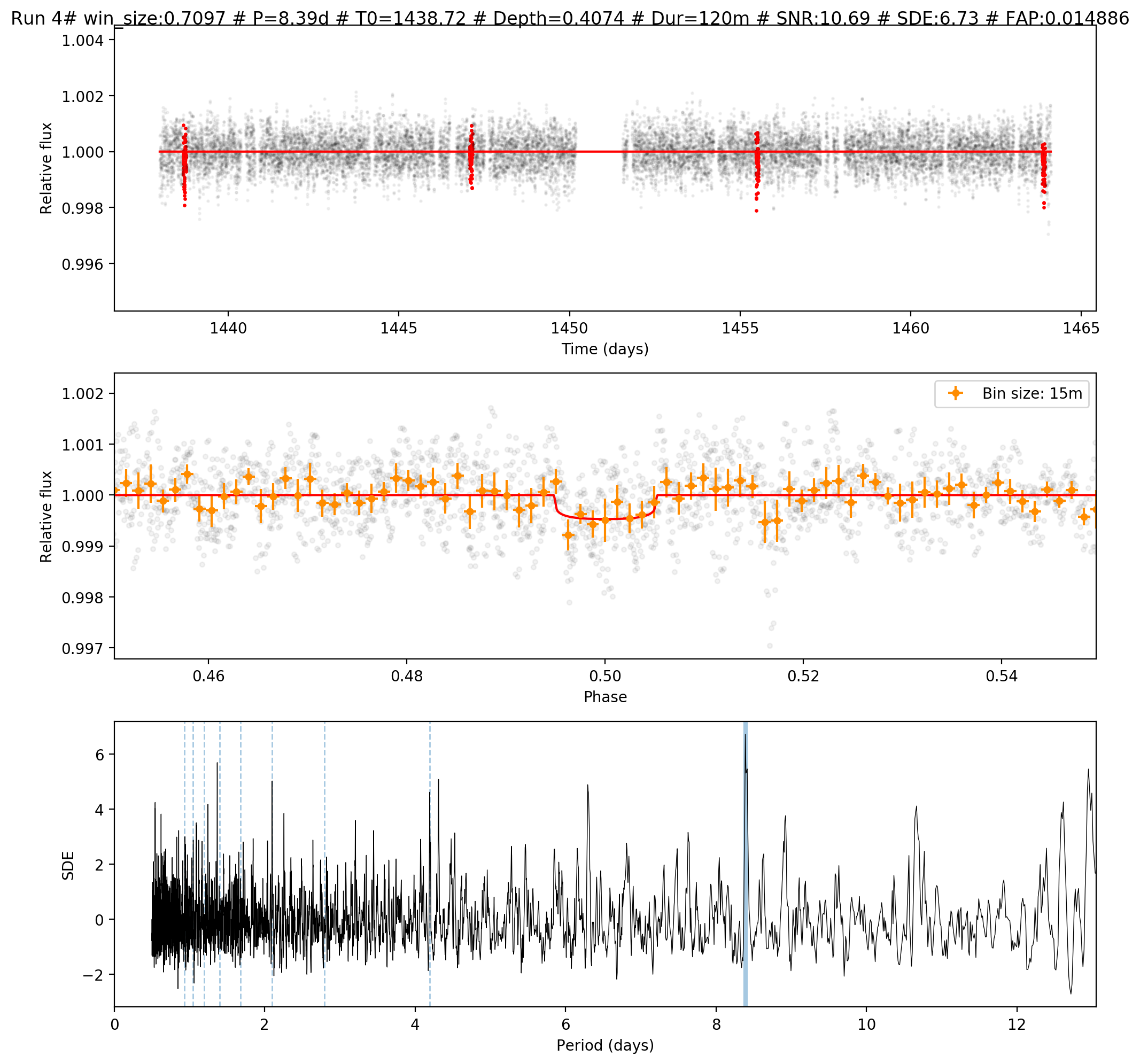
It does not look bad. Let us now have a look at the full set of results from RUN 4, where this candidate was found (available in the TIC259377017_[5]_report.log):
________________________________ run 4________________________________
=================================
MODELS IN THE DETRENDING - Run 4
=================================
light_curve              Detrend_method   win/ker_size   RMS (ppm)  RMS_10min (ppm)
PDCSAP_FLUX_4            ---              ---            595.39     488.76
flatten_lc & trend_lc 0  biweight         0.2457         576.86     470.91
flatten_lc & trend_lc 1  biweight         0.3617         581.15     476.91
flatten_lc & trend_lc 2  biweight         0.4777         582.09     477.80
flatten_lc & trend_lc 3  biweight         0.5937         583.32     478.33
flatten_lc & trend_lc 4  biweight         0.7097         584.15     479.32
flatten_lc & trend_lc 5  biweight         0.8257         585.10     480.30
flatten_lc & trend_lc 6  biweight         0.9417         585.81     481.00
flatten_lc & trend_lc 7  biweight         1.0577         585.75     481.14
flatten_lc & trend_lc 8  biweight         1.1737         585.21     480.48
flatten_lc & trend_lc 9  biweight         1.2897         585.48     480.64
flatten_lc & trend_lc 10 biweight         1.4057         585.92     481.35
flatten_lc & trend_lc 11 biweight         1.5217         586.10     481.42
=================================
SEARCH OF SIGNALS - Run 4
=================================
win_size    Period    Per_err   N.Tran  Mean Depth (ppt)  T. dur (min)  T0            SNR           SDE           FAP           Border_score
PDCSAP_FLUX 12.99591  inf       1       0.658             239.3         1450.9798     11.969        16.236        8.0032e-05    0.00
0.2457      3.44744   0.006321  8       0.400             72.4          1439.1505     9.823         5.920         0.064745898   0.88
0.3617      4.31143   0.008517  6       0.412             62.2          1438.0330     8.588         5.449         nan           0.83
0.4777      8.38974   0.029009  4       0.392             119.7         1438.7234     10.312        6.332         0.031132453   1.00
0.5937      8.38974   0.029009  4       0.401             119.7         1438.7234     10.545        6.623         0.017767107   1.00
0.7097      8.38974   0.024849  4       0.407             119.7         1438.7234     10.691        6.728         0.014885954   1.00
0.8257      12.95153  0.059124  2       0.599             90.1          1438.0198     9.405         6.775         0.01392557    0.50
0.9417      12.95153  0.059124  2       0.675             90.1          1438.0198     10.586        8.190         0.001040416   0.50
1.0577      12.95153  0.066565  2       0.699             90.1          1438.0198     10.965        8.628         0.00040016    0.50
1.1737      12.99591  0.066565  1       0.484             197.8         1450.9892     8.112         9.181         8.0032e-05    0.00
1.2897      12.99591  inf       1       0.497             197.8         1450.9892     8.335         9.391         8.0032e-05    0.00
1.4057      12.99591  inf       1       0.507             197.8         1450.9892     8.491         9.323         8.0032e-05    0.00
1.5217      12.99591  inf       1       0.523             197.8         1450.9892     8.759         9.635         8.0032e-05    0.00
Elected signal with QUORUM algorithm from 3 VOTES --> NAME: 4	Period:8.389738737546075	CORR_SNR: 12.33603015435488	SNR: 10.69122613377423	SDE: 6.727610929963518	FAP: 0.014885954	BORDER_SCORE: 1.0
Proposed selection with BASIC algorithm was --> NAME: PDCSAP_FLUX	Period:12.995907399200522	SNR: 11.968942425672902
New best signal is good enough to keep searching. Going to the next run.
One hint to identifying false positives is the number of times that the signal was recovered. Real planetary signals tend to be recovered by many different detrends. In our case, the signal is recovered three times only, and is in competition with another signal whose period is 12.99 days. However, this was neglected by the quorum algorithm because it was highly affected by the borders (look at that border score!). The signal of 8.39 days, which although it initially look promising, its SDE is very low, below 9 or 10, which is suspiciously low. Moreover, the FAP is high. These values make us think that it could be just noise. But if you still want more proof, you can use the vetting tool, and
if still looks acceptable, you can perform a fit and try to obtain follow-up observations to procure high-precision photometry to confirm the signal. In this particular case, the depth of the signal is very shallow (only ~0.4ppt), which is very challenging for current
ground-based telescopes!. Unfortunately, in our opinion, this signal is not worth following-up, but of course judge for yourself with your own candidates!